Lesson 8 - Simulating a Forecast with an Information Delay

In Lesson 6, we noted that models of engineering systems may sometimes need to use Information Delays (e.g., to represent reporting delays). However, unlike business models, in most cases, engineering models would be based on measured (as opposed to perceived) signals, and hence these Information Delays would have zero Dispersion.  However, there is one very important use for Information Delays with Dispersion that can be useful in both business models and engineering models that we will discuss in this Lesson.

Many decisions (e.g., how to adjust a pumping rate, how to change a production rate) are based on forecasts of future behavior (e.g., the expected inflow rate, the expected sales rate) based on past observations. A forecast can help improve decision making.  For example, when trying to use a Controller in a feedback control system that is trying to control a volume in a pond, we should be able to do a better job if we can forecast what the uncontrolled inflows and outflows to the pond will be that will also impact that volume. In order to simulate such systems using GoldSim, it is necessary to simulate the forecasting process itself.

An Information Delay can be used to represent a very commonly used forecasting method known as exponential smoothing. In exponential smoothing, the forecast is based on an exponentially-weighted average of past observations. Mathematically, this is equivalent to the output of an Information Delay with a Dispersion (Erlang n) equal to 1: 

When using an Information Delay to simulate an exponentially smoothed forecast, the Delay Time is a measure of how heavily weighted previous values are. The larger the Delay Time, the more heavily weighted older values are (i.e., the farther the forecast reaches back in time to generate the forecasted value). The smaller the Delay Time, the more heavily weighted more recent values are. A larger Delay Time will generally result in a smoother forecast, but one that is less responsive to the most recent values. A smaller Delay Time will generally result in a noisier forecast, but one that is very responsive to the most recent values.

 An example of such a simulated forecast is presented below:

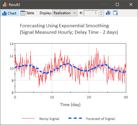
In this case, there is a very noisy input to the Information Delay, and the Delay Time is 2 days.

In the next Lesson we will work on an Exercise in which we use such a forecast to improve the performance of a feedback control system using a Proportional Controller.