Lesson 6 - Modeling Information Delays

Information Delay elements are intended to be used to simulate delays in measuring, reporting, and/or responding to information. Such delays exist because it invariably takes time to collect, assimilate and act on new information.

Reporting yesterday’s rainfall total today is an example of an information delay, with a delay time of one day. In the business world, a classic example of an information delay is the delay in perceiving a change in a variable.

Note that the reported or perceived value (i.e., the output of the Information Delay) is computed based on the historical values of its inputs.  Because Information Delays usually represent processes such as perception, measurement and reporting, by definition, these elements are typically used to simulate human actions. In particular, they are often used to represent the decision-making process of someone (or some group) in the system being simulated.

Note that unlike Material Delays (in which material is conserved as it moves through the Delay), that is not the case for Information Delays.  Information is a signal  at a particular time; it is not material.  As such, "conservation" of the signal does not really apply as it moves through the Delay.  Hence, whereas integrating the output of a Material Delay produces the amount of material that has left the Delay, integrating the output of an Information Delay is not really meaningful.

In order to understand how an Information Delay works, let’s open a simple pre-built model. To do so, go to the “Examples” subfolder of the “Basic GoldSim Course” folder you should have downloaded and unzipped to your Desktop, and open a model file named Example13_InformationDelay.gsm.  The model contains two different Information Delays and looks like this:

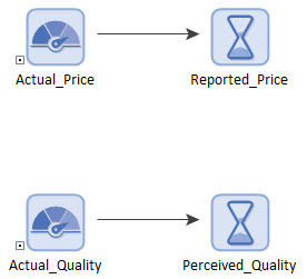
Let's first look at the one on the top.  In this example, we are tracking the price of an item (e.g., at a store).  The Actual_Price represents the actual price of the item.  This price can change at any time.  However, it takes 5 days for any new prices to be reported (e.g., it takes 5 days to record and ultimately transmit that information).

Open the Reported_Price Information Delay:

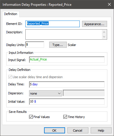
The element requires an Input Signal (in this case, the Actual_Price). The Delay Time determines how long it takes to transit the Delay. That is, how long any changes to the Input Signal are delayed until it is reported.  In this case, it takes 15 days.

Run the model and look at the result (the Prices Time History Result element):

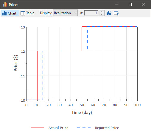
The result here is pretty simple.  The Reported Price always lags the Actual Price by 5 days.  How could this affect a model? Decisions are made based in the Reported Price (as that is the only information the decision maker has). As we will see in the next Lesson, this can have important impacts on other parts of a model (e.g., feedback control systems that are controlled by the price).

Now let's look at the second example.  This one is slightly different (and more complicated). In this example, we are tracking the quality some product. For simplicity here, the quality is represented by a number (the higher the number, the higher the quality). The customers' perception of the quality is driven by word of mouth (e.g., online reviews). What we are interested in is the customers' perception of the quality (as this will affect sales). If you think about it, changes in the perceived quality of the product will necessarily lag any changes in the actual quality of the product.  Moreover, if the quality of the product changes suddenly, we would not expect the customers' perception to change suddenly.  Rather, we would expect it to change gradually (e.g., as more positive online reviews accumulate).  We can simulate this process by using an Information Delay with Dispersion.

Open the Perceived_Quality Information Delay: 

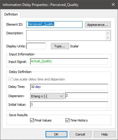
The Input Signal is the Actual_Quality. The Delay Time is set to 10 days (there is a lag in how the perception of the quality changes). In addition, we have specified a Dispersion. As we shall see, this results in the perceived quality changing gradually.

Note: The degree of Dispersion can be represented in two different ways: by specifying a “Standard Deviation”, or by specifying an “Erlang n”.  GoldSim Help explains how one relates to the other.

Let's look at the result (the Quality Time History Result element):

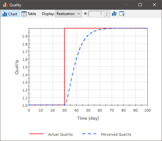
As can be seen, the actual quality changes suddenly (going from 1 to 2 at 30 days).  However, the perceived quality changes gradually, taking 30 or 40 days to reflect the actual quality.  How could this affect a model?  Again, some decisions that you may be simulating may be made based not on the actual quality, but on the perceived quality (e.g., ramping up production rate for anticipated sales).

It would not be unusual for models of engineering systems to use Information Delays (e.g., to represent reporting delays).  However, in most cases, engineering models would be based on measured (as opposed to perceived) signals (and hence would have no Dispersion).  Modeling perceptions like we did above is much more common in business models.  However, there is one very important use for Information Delays with Dispersion (for both business models and engineering models) that we will discuss in Lessons 8 and 9.