Lesson 9 - The Proportional Controller

The Controller has three different (user-selected) control methods by which it determines the Controller output. In the previous Lesson, we looked at one of the those methods (a Deadband Controller). As we saw, the Deadband Controller produces an output that switches abruptly between two states: a specified flow (the Flow Capacity) or zero flow. That is, it does not adjust flows in a continuous manner; it simply abruptly turns flows on and off.

In some systems, however, you may want to have your Controller respond in a continuous and gradual manner:

• In some cases, the control system you are trying to represent may actually respond continuously (or near continuously): it automatically and continuously adjusts inflows/outflows (e.g., by changing a pumping rate or controlling a valve) in response to the current value of the process variable.
• In other cases, the system is not actually continuously adjusted in real time, but over the timescale of interest, can effectively be considered to respond in a gradual and continuous manner. That is, you are not necessarily trying to explicitly represent the control process in a detailed way. Instead, what you want to do is represent the “lumped effect” of the various actions taken by the system’s operator that result in a system that smoothly approaches and closely tracks the target.

In both of these cases, we need a Controller that responds smoothly (as opposed to abruptly like the Deadband Controller). In this Lesson, we will explore a second type of Controller that supports such a response: the Proportional Controller.

In order to illustrate how a Proportional Controller works, we will look at a simple example. Go to the “Examples” subfolder of the “Basic GoldSim Course” folder you should have downloaded and unzipped to your Desktop, and open a model file named Example5_Proportional_Controller.gsm.

In this model, a Pond starts at a volume of 200 m3 and has a constant uncontrolled inflow of 5 m3/day (i.e., you have no control over this inflow). We want to use an Outflow Controller to adjust the outflow rate so that the pond gradually and smoothly approaches a target volume of 50 m3.

A Proportional Controller continuously adjusts the output such that it is proportional to the current error.

The error is the difference between the current value of the process variable and the target. Hence, unlike the Deadband Controller (whose output is either zero or a specified value), the output of a Proportional Controller can vary continuously between some maximum value and zero.

How the error is calculated is a function of whether the Controller is an Inflow or Outflow Controller:

• Outflow Controllers: Error = Process Variable – Target
• Inflow Controllers: Error = Target – Process Variable

The output is then computed as follows:

Output = Min (Max (Bias + Proportional Gain*Error, 0), Flow Capacity)

As indicated by the equation, GoldSim starts by computing the output as Bias + Proportional Gain*Error. That is, the output is linearly proportional to the error. Note, however, that there are two constraints imposed:

• The output cannot be less than zero. This could happen if the Error was sufficiently negative.
• There is a maximum value for the output (the Flow Capacity). In this example, the Flow Capacity is 25 m3/day.

Hence, when you select “Proportional” as the Method, there are three additional inputs that must be provided: the Target, the Bias and the Proportional Gain:

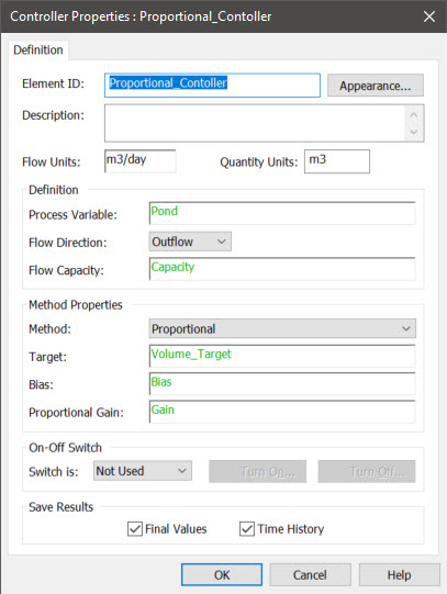
The Target, of course, is the value you are trying adjust the Process Variable toward (in this example, 50 m3). The Bias is the value of the output when the error is zero (i.e., it has the same dimensions as the Process Variable). The Proportional Gain has dimensions of inverse time, and represents how strongly the Controller responds to the error. The larger this number, the quicker it responds. The Bias and Proportional Gain can be thought of as “tuning parameters”. That is, you will need to experiment with these two parameters to achieve the performance you desire.

Let’s run this model and view the time history result:

As can be seen, the volume gradually and smoothly approaches the target.

This example is very simple in that the uncontrolled inflow rate that the Controller is trying to compensate for to adjust the volume is constant. In most models, this will not be the case. That is, there will be uncontrolled inflows and/or outflows impacting the process variable (in this case, the volume in a pond) and these will likely be variable instead of constant.

To illustrate this, let’s consider another example. Go to the “Examples” subfolder of the “Basic GoldSim Course” folder you should have downloaded and unzipped to your Desktop, and open a model file named Example6_Proportional_Controller.gsm.

This example is identical to the previous example with three differences:

• The model is run for 200 days (instead of 100 days).
• The initial volume in the pond is 50 m3 (i.e., it is at the target value).
• The inflow rate is not constant, but varies considerably (slowly oscillating and increasing).

Let’s run this model and view the time history result:

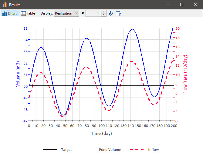
As can be seen, the Controller is unable to effectively manage the volume and return it to the target. It oscillates (like the inflow rate) around the target, and increasingly diverges from it.

Clearly, in a situation like this, the Proportional Controller is not effective. Fortunately, there are two different ways to address this and get better performance. One is to improve the way we specify the two tuning parameters (the Bias and the Proportional Gain). In particular, in order for the Proportional Controller to perform well in this situation, we need to define the Bias as being time-variable (instead of constant). We will discuss the best way to do that in the next Unit (Unit 9, Lesson 9). A second way to improve this performance is to use a different Controller method: the PID Controller. We will discuss this in the next Lesson.