Lesson 8 - The Deadband Controller

As discussed in the previous Lesson, in many systems there is active feedback control designed directly into the system to make it behave in a specified manner. While feedback control logic can be represented in GoldSim using basic GoldSim elements, the Controller element makes it much easier to build and represent such logic while also enforcing a consistent methodology and removing difficulties users can face when building the logic from scratch with basic elements.

Controllers use feedback control to influence the state of a “process” and adjust it to a desired value (a target). A “process” could conceptually involve something quite complex (e.g., an entire chemical plant), but typically will be something much more specific (e.g., a single tank in that plant). The state is some property of the process that we want to control (e.g., the volume of water in the tank). The state is referred to as the process variable. In GoldSim, the process variable is usually the main output of a Pool or Reservoir (and hence a state variable). Recall that state variables were defined in Lesson 3.

Controllers produce a single output which is always a flow of some kind (e.g., an inflow or outflow of water, heat, mass, items, etc.). This flow is then intended to be connected back to the process (e.g., a Pool element representing the volume of water in a tank) in order to adjust the value toward the target. The key point here is that the Controller requires as input a process variable (which will typically be the primary output of a Pool or Reservoir) and in turn produces a flow that is then directed back to impact that process variable (e.g., an inflow or an outflow to the Pool or Reservoir defining the process variable). This forms a feedback loop:

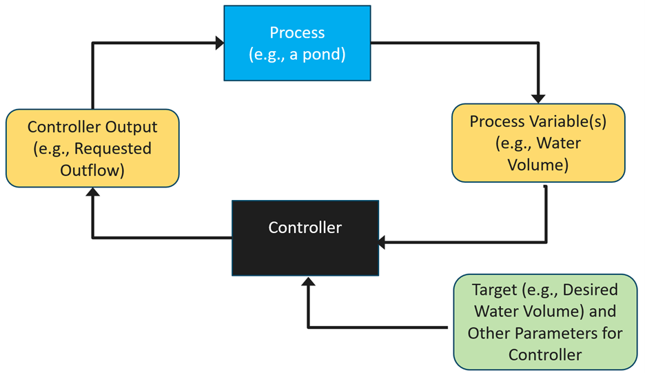
The goal of the Controller is to produce an output that when fed back into the process directs the process variable back toward the target. The Controller has three different (user-selected) control methods by which it determines the Controller output. This Lesson introduces one of those methods: the Deadband.

Controllers are defined as either Inflow Controllers or Outflow Controllers. This determines if they are intended to respond in order to decrease the process variable (an Outflow Controller) or to increase the process variable (an Inflow Controller). This means that they are uni-directional (a Controller can only act in one direction: it can either act to increase the process variable or to decrease it). As their names indicate, the output of an Inflow Controller is intended to be used as an inflow to the process (e.g., an inflow to the Pool or Reservoir being controlled), while the output of an Outflow Controller is intended to be used as an outflow to the process (e.g., an outflow request to the Pool or Reservoir being controlled).

The easiest way to start to understand a Controller is to look at a simple example. In particular, we are going to revisit an example we looked at in the previous Lesson. You should recall that in that model, we turned a pump on and off when the water volume in a pond reached a specified target (300 m3). However, the simplistic way in which we did that resulted in a system in which the outflow oscillated rapidly. We pointed out in that Lesson that the system would never be designed to operate like this in the real world. If it did, the pump would be turning on and off every few seconds!

This example uses a Controller to more realistically control the water volume. Go to the “Examples” subfolder of the “Basic GoldSim Course” folder you should have downloaded and unzipped to your Desktop, and open a model file named Example4_Deadband_Controller.gsm.

This model is identical to the previous Example (Example3_Feedback_Control), with one exception: the simple Expression element defining the withdrawal from the Pond (Withdrawal) is replaced by a Controller element.

Open the Controller (named Deadband_Controller):

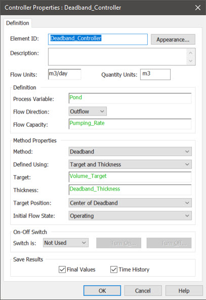
All Controllers have the following common inputs (at the top of the dialog):

Display Units: These are the display units for the output of the Controller. Note that this output should be a flow rate of some kind (in this case it is a volumetric flow).

Process Variable: This is the variable that is being monitored and controlled by the Controller. In this case, it is the primary output of the Pond (a Pool element). It has dimensions of Display Units * Time. In this case, it is a volume.

Flow Direction: Either “Inflow” or “Outflow”. In this example, this is an Outflow Controller (i.e., it will control an Outflow Request from the Pool).

Flow Capacity: This is the maximum value that the output of the Controller can take on. It is typically associated with some physical limitation (e.g., the size of a pump). In this case, we have assigned it a value of 200 m3/day (which is higher than the inflow rate of 100 m3/day).

The Controller provides three different (user-selected) control methods by which it determines the Controller output. Depending on the method selected, the required inputs (and hence the dialog) will change.

In this example, the Controller uses the Deadband method. A Deadband Controller produces an output that switches abruptly between two states: a specified flow (the Flow Capacity) or zero flow. When you select “Deadband” as the Method, there are two ways to define it (Defined Using): by specifying a "Target and Thickness", or specifying the "Top and Bottom" of the Deadband. In this example, the former manner of defining the Controller is used. There are three key inputs that must be provided: the Target, the Thickness and the Target Position.

The Thickness defines the size of the range between which the process variable is controlled. The Target lies either halfway between the upper and lower boundaries of this band, or at one of the boundaries of the band (as determined by the Target Position). In this case, the Target is defined as 300 m3 and the Thickness is defined as being 10 m3, and the Target Position is “Center of Deadband”. As a result, the process variable is controlled between 295 m3 and 305 m3. In particular, when the process variable reaches the top of the deadband, the output is set to the Flow Capacity. When the process variable reaches the bottom of the deadband, the output is set to zero.

Run the model and view the time history result:

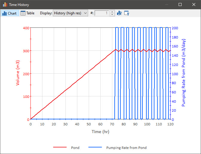
The volume “bounces” around the target (between 295 m3 and 305 m3). More importantly, rather than oscillating continuously on and off, the pump is turned on and off in a controlled (and relatively infrequent) manner. That is, by definition, the flow rate still oscillates on and off, but does so in a controlled manner (with the size of the deadband and the Flow Capacity controlling the period of oscillations). The smaller the deadband and higher the Flow Capacity, the more frequent the oscillations. As a result, the deadband is typically defined to be large enough to limit the frequency of oscillations.

It should be noted that you likely utilize a Deadband Controller in the real world all the time. A thermostat is essentially a Deadband Controller (e.g., it turns the furnace on when the temperature drops to one level, and turns it off when it reaches some higher level). You don’t actually define the deadband yourself. Instead, you set the target temperature in the thermostat, and it automatically assigns a deadband around it.

Note: In this example, because the pump was turned on at 305 m3 does not mean that the volume cannot exceed that value. In this example, the inflow is constant (and always less than the Flow Capacity). But if the inflow was variable, it could perhaps at least temporarily exceed the pumping rate (in which case the volume would temporarily go beyond the top of the deadband). If you truly needed to ensure that the volume never exceeded 305 m3, you would need to turn the pump on before it reached that volume and/or the Flow Capacity would need to be such that it was always higher than the inflow (which in a real system of course would be unlikely to be constant).

Note: If you were actually trying to control the volume of water in a pond like this, the triggers to turn the pump on and off would not be the volume (as this is typically not something that can easily be monitored). Rather, it would be the water level. In this case, the Process Variable would still be a volume, but the deadband would be defining by specifying the top and bottom.  You would then define these as water levels, which you would then convert to volumes (e.g., using a Lookup Table) such that the top and bottom of the deadband could then be specified in the Controller dialog as volumes.

This simple example (and those we will discuss in later Lessons) uses an Outflow Controller. However, depending on the process, you may need just an Outflow Controller, just an Inflow Controller, or both. For example, if a pond had inflows that you had no control over (e.g., rainfall), and you had a pump that you could control to respond to those inflows and maintain a target water level (by removing water), you would need an Outflow Controller. That is what this simple example model did. On the other hand, if a pond had outflows that you had no control over (e.g., evaporation), and you had a pump that you could control to respond to those outflows and maintain a target water level (by adding water), you would need an Inflow Controller. Finally, if you had a pond that had both inflows (rainfall) and outflows (evaporation) that you had no control over and you had one pump that you could control to remove water when needed and one pump that you could control to add water when needed, you would need both an Inflow Controller and an Outflow Controller (i.e., a Controller for each pump).

As noted above, the Controller has three different (user-selected) control methods by which it determines the Controller output. In this example, we looked at one of those methods (a Deadband). We will look at another method in the next Lesson.