Lesson 11 - Using Feedback Control and Allocation to Realistically Represent Outflows

Now that we have covered the use of the Controller element for representing feedback control, we are finally ready to complete a discussion regarding the representation of outflows from a stock of material that we started in Unit 7 (Lessons 11, 12 and 13).

In Lesson 8, we examined a feedback control problem in which the goal was to control a state variable (i.e., the water volume) around a particular “target” level.  We accomplished this by implementing a deadband using a Controller element.

Although this is a common objective (e.g., a thermostat does this), it is also quite common for feedback control systems to be used to control the behavior of a system as it approaches its physical bounds (e.g., controlling the pumping rate to or from a pond as it approaches its upper limit or as it empties). One way to do this, of course, would be simply to have your “band” adjacent to the bound (e.g., turn a pump off when the volume reaches 0 m3 and turn it back on when the volume reaches, say 5 m3).

However, some systems may not work in such a binary manner.  Instead, they may gradually adjust flows as the volume approaches the bounds.  For some flows, this could happen naturally (e.g., as the volume decreases, the surface area decreases, and hence the evaporation rate decreases, going to zero as the volume goes to zero).  In other cases, you might intentionally slowly adjust the flows as you approach a bound (e.g., decreasing a pumping rate gradually as the volume approached zero). We discussed how this might be done in Lesson 9 using a Proportional Controller.

In addition, as we saw in Unit 7, Lesson 13, in a situation where the outflows from a stock of material must be constrained (because Requested Outflows exceed Inflows, and the stock is at its lower bound), it becomes necessary to prioritize and allocate any remaining (i.e., non-zero) Requested Outflows.  We saw that a Pool element supports such prioritization.

In many systems, in order to be realistically represented, different outflows would likely need to be treated in different ways as the bound is approached: some would need to be turned off (e.g., using a Deadband Controller), others would need to gradually be changed (e.g., using a Proportional Controller), and others would need to be prioritized (and hence reduced perhaps) once the bound is reached (and outflow is constrained). To illustrate this, in this Lesson, we are going to look at an Example that deals with multiple outflows, each of which needs to be represented differently. 

The model can be found in the “Examples” subfolder of the “Basic GoldSim Course” folder you should have downloaded and unzipped to your Desktop.  In that folder, open a model file named Example8_Multiple_Outflows.gsm.  The model looks like this:

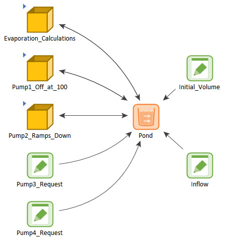
The model is relatively complex compared to the Exercises we have done, but is still quite simple.  It utilizes some Containers to organize the model.  The model simulates a pond that has an initial volume of 200 m3 with a constant inflow (10 m3/day).  It has five outflows:

• Water evaporates from the pond.  The rate of evaporation is proportional to the pond surface area.  The surface area is a function of the pond volume (and this relationship is represented by a Lookup Table).  The Evaporation_Calculations Container contains the elements that compute the evaporation.  If you explore that Container, you will see that this is the identical structure that was used in Exercise 8 (Unit 8, Lesson 6).  The evaporation goes to zero as the volume goes to zero.  This is an example of a passive (natural) feedback control mechanism.
• Pump1 is actively turned off (and on) based on a deadband. It initially pumps at a constant rate (of 20 m3/day).  However, it is switched off when the pond volume decreases to a certain level (100 m3).  If the pond volume were to rise (above 110 m3) it would turn on again.  The Pump1_Off_at_100 Container contains the elements that control the pumping rate.  If you explore that Container, you will see that it uses a Deadband Controller element. The pumping rate becomes zero well before the pond volume reaches zero. This is an example of an active feedback control mechanism utilizing a deadband.
• Pump2 ramps down gradually. The pumping rate is proportional to the volume of water in the pond.  However, the pump has a capacity of 10 m3/day, so at early times it is limited to that rate.  If you explore that Container, you will see a Proportional Controller (with a Target of 0 m3) is used to control the pumping rate. The pumping rate goes to zero as the volume goes to zero.  This is an example of an active feedback control mechanism in which the rate is gradually and smoothly adjusted.
• Pump3 and Pump4 are defined using constant Outflow Requests (of 8 m3/day).  As a result, no explicit measures are taken to reduce their values when the pond volume goes to zero. However, if the pond goes empty, the total outflow must be constrained (it could not be greater than the inflow, which is 10 m3/day). In this case, the actual outflows for Pump3 and Pump4 must be adjusted.  Physically, this is equivalent to saying that when the outflow becomes constrained, we will instantaneously adjust Pump3 and Pump4 accordingly. In order to do so, of course, we need to define some priorities.  Conceptually, this too is a form of feedback control (the actual pumping rates are reacting to the pond volume), but it is done internally to the Pool element, so it is not as evident.

Note: If you were actually trying to control the volume of water in a pond like this, Pump1 and Pump2 would not likely respond to the volume (as this is typically not something that can easily be monitored).  Rather, they would respond to the water level (which would typically be computed from the volume using a Lookup Table).

Let’s look at the Outflows tab of the Pool representing the pond:

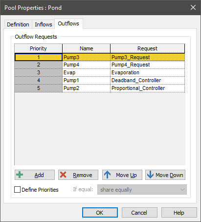
We know from the discussion above that the evaporation, Pump1 and Pump2 are all zero when the pond volume goes to zero.  But that is not the case for Pump3 and Pump4.  The Outflow Requests are constant, and hence if the pond goes to zero (and as we shall see, it does), those two flows need to be constrained. As can be seen here, Pump3 has a higher priority than Pump4.  (The priorities of the other Outflows are lower, but their priorities are inconsequential, as their Requests are all zero if the outflow becomes constrained due to the volume going to zero.)

Run the model and display the results (by double-clicking on the Time History Result element):

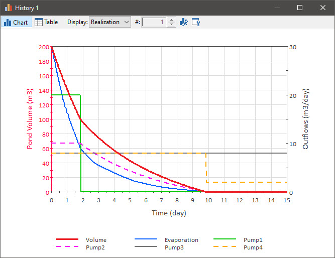
The pond volume is plotted on the left-hand axis (it is a thick red line), and all of the flows are plotted on the right-hand axis. Note that the pond volume goes to zero just before 8 days.  Let’s examine the five outflows:

• The evaporation gradually decreases with the pond volume, going to zero when the pond volume goes to zero.
• Pump1 turns off (suddenly) when the pond volume reaches 100 m3.
• Pump2 is initially limited to a pumping rate of 10 m3/day, and then gradually decreases with the pond volume, going to zero when the pond volume goes to zero.
• Pump3 stays constant during the entire simulation.  Pump4, however, immediately drops from 8 m3/day to 2 m3/day when the pond goes empty.  This is because the outflow becomes constrained, and Pump3 has a higher priority than Pump4.

This is obviously a simplistic and artificial example, but is serves to illustrate the different ways that you can use feedback control and the allocation/prioritization capabilities of the Pool element to represent multiple (and potentially competing) outflows.

The key point that you should take away from this discussion is that when building a model that involves outflows that have active or passive feedback control, it is critical for you have a very good understanding of how the real system actually works such that you represent realistic control systems in your model (i.e., systems that could be practically implemented). Otherwise, your simulated predictions will behave unrealistically and/or be of very limited value.