Lesson 10 - The PID Controller

The Controller has three different (user-selected) control methods by which it determines the Controller output. In the previous Lesson, we looked at the second of those methods (a Proportional Controller). As we saw, the Proportional Controller performs well under some circumstance, but performs poorly under others (i.e., when the uncontrolled inflows/outflows are highly variable).

As we shall see, the PID (Proportional Integral Derivative) Controller performs quite well under these circumstances. Like the Proportional Controller, it continuously adjusts the output as a function of the error. Unlike that Controller, however, in which the adjustment is a simple function of the error, the adjustment for a PID Controller depends not only on the error, but on the integral and derivative of the error. This makes it more powerful (but as we shall see, it requires more tuning parameters).

In order to illustrate how a PID Controller works, we will look at a simple example. Go to the “Examples” subfolder of the “Basic GoldSim Course” folder you should have downloaded and unzipped to your Desktop, and open a model file named Example7_PID_Controller.gsm.

This is identical to the previous example, except instead of using a Proportional Controller, we use a PID Controller. Recall that in this model, a Pond starts at a volume of 50 m3 (the target), and the inflow rate is not constant, but varies considerably (slowly oscillating and increasing).

Like the Proportional Controller, a PID Controller continuously adjusts the output as a function of the error.

As is the case for the Proportional Controller, the error is the difference between the current value of the process variable and the target. How the error is calculated is a function of whether the Controller is an Inflow or Outflow Controller:

• Outflow Controllers: Error = Process Variable – Target
• Inflow Controllers: Error = Target – Process Variable

The output is then computed as follows:

Output = Min (Max (Bias + PID Sum, 0), Flow Capacity)

where PID Sum is the sum of three different terms:

\(\mathrm{\displaystyle PID\ Sum=P+I+D}\)

 \(\mathrm{\displaystyle P=Proportional\ Gain*Error}\)

  \(\mathrm{\displaystyle I=Integral\ Gain*\int\limits_0^{Etime}Error\ dt}\)

  \(\mathrm{\displaystyle D=Derivative\ Gain*\frac{dError}{dt}}\)

As indicated by the equation, GoldSim starts by computing the output as Bias + PID Sum. Note, however, that there are two constraints imposed:

• The output cannot be less than zero. This could happen if the Error was sufficiently negative.
• There is a maximum value for the output (the Flow Capacity). In this example, the Flow Capacity is 25 m3/day.

Hence, when you select “PID” as the Method, there are five additional inputs that must be provided: the Target, the Bias, the Proportional Gain, the Integral Gain and the Derivative Gain:

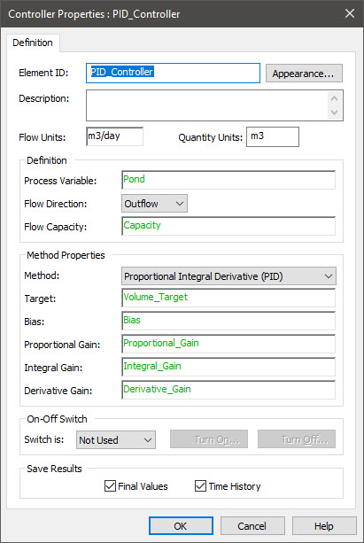
The Target, of course, is the value you are trying adjust the Process Variable toward (in this example, 50 m3). The Bias is the value of the output when the PID Sum term is zero (which can be non-zero even if the error itself is zero). It has the same dimensions as the Process Variable. The Proportional Gain has dimensions of inverse time, and represents how strongly the “P” term in the sum responds to the error. The Integral Gain has dimensions of the inverse time squared, and represents how strongly the “I” term in the sum to responds to the integral of the error. The Derivative Gain is dimensionless, and represents how strongly the “D” term in the sum responds to the derivative of the error. The Bias, Proportional Gain, Integral Gain and Derivative Gain can be thought of as “tuning parameters”. That is, you will need to experiment with these four parameters to achieve the performance you desire.

Let’s run this model and view the time history result:

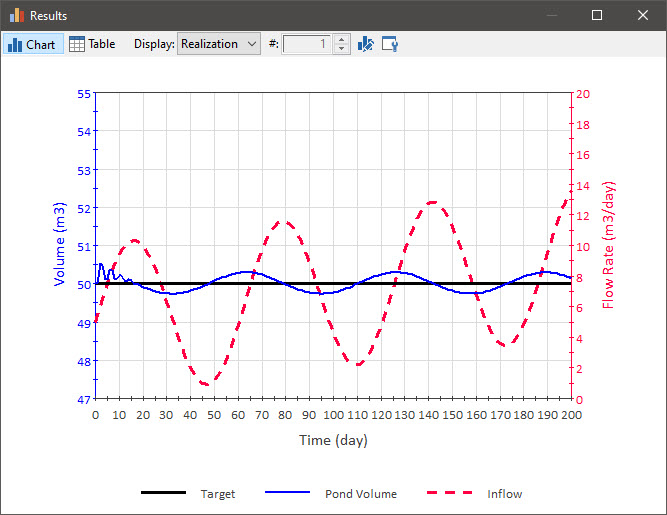
As can be seen, the Controller is able to effectively manage the volume and return it to the target. It does oscillate (like the inflow rate) slightly around the target, but tracks it closely.

Clearly, in a situation like this, the PID Controller is much more effective than a Proportional Controller. Of course, the PID Controller requires four tuning parameters, and hence takes a bit more effort to “tune”. As noted in the previous Lesson, another way to address such a complex system is to use a Proportional Controller with a time-variable Bias. We will discuss that approach in the next Unit (Unit 9, Lesson 9).