Lesson 1 - Unit 12 Overview

"We must become more comfortable with probability and uncertainty."

- Nate Silver

In the previous Unit we introduced the fundamental concepts of probabilistic simulation, and started to describe GoldSim’s capabilities for representing uncertainty in our models. In this Unit, we will continue to explore these capabilities.

The first half of this Unit will focus on how GoldSim can be used to represent stochastic processes. A stochastic process is a process that is inherently random, but changes over time according to some probabilistic rules. That is, the temporal behavior of the system cannot be predicted precisely, but can be described statistically.  Examples of such processes include stock market fluctuations, rainfall, and Brownian motion.

Recalling our discussion from the previous Unit, we noted that when quantifying the uncertainty in a system, there are two fundamental causes of uncertainty that it is important to distinguish between:

1. that due to inherent (temporal) randomness; and
2. that due to ignorance or lack of knowledge.

A stochastic process is another way to refer to the first type of uncertainty. That is, a variable that exhibits the first type of uncertainty can be said to behave stochastically. In the previous Unit, we showed how GoldSim could be used to represent the second type of uncertainty (that due to ignorance or lack of knowledge). In this Unit we will focus in detail on how GoldSim can be used to represent the first type of uncertainty (that due to inherent randomness or stochasticity).

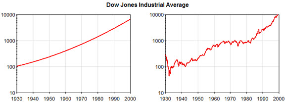
The reason that this is so important is that many (if not all) complex, real-world processes behave stochastically to some extent.  As a very simple illustration, consider the following two time histories (representing the value of the Dow Jones Industrial Average from 1930 to 2000):

Even if someone knew nothing about the stock market (and therefore did not understand that it fluctuates significantly), which would they think looks more realistic?  Of course it would be the second one.  That is, even though we can often think about and describe processes approximately using a relatively simple model (in this case, a geometric growth rate), it is intuitive to most people that the real world usually does not follow such smooth curves. This is because our daily observations of the world indicate to us that many processes and systems are “noisy” (i.e., they behave stochastically to some extent).

In many systems, it is critical to represent this “noisy” behavior (particularly when carrying out risk analysis), as ignoring it (by assuming the system behaves in an “averaged” or “smoothed” manner) can often lead to poor decision making.  As a very simple example, you would never design a seawall based on the highest predicted tide.  You would also account for random fluctuations that could be superimposed on that tide (e.g., due to storms).

After first focusing on how GoldSim can be used to represent stochastic processes, we will conclude the Unit by discussing several advanced probabilistic modeling features. In particular, in this Unit we will discuss the following:

• Representing a stochastic process: resampling a Stochastic;
• Autocorrelating a Stochastic;
• Using the Extrema element;
• Representing a stochastic process: randomly sampling a time series;
• Understanding random numbers and sampling;
• Determining how many realizations are necessary;
• Classifying and screening realizations;
• Viewing distribution results at different times in a simulation; and
• Running a deterministic simulation with uncertain inputs.

This Unit also includes two Exercises (in addition to a number of Examples that we will work through together). This Unit has a total of 12 Lessons (including this overview and a summary at the end).